on
Fast Fourier Transform (FFT)
Fast Fourier Transform
Given two polynomials
\[A(x)=x^2+3x+2\quad\quad B(x)=2x^2+1\]The coefficients of \(A\) and \(B\) is respectively \([1, 3, 2]\) and \([2,0,1]\). A multiplication of the two polynomials can be represented as
\[\begin{align} C(x)&=A(x)\cdot B(x)\\ &=2x^4+6x^3+5x^2+3x+2\longrightarrow C=[2,6,5,3,2] \end{align}\]If \(A=[a_0,a_1,...a_d]\), \(B=[b_0,b_1,...b_d]\), then runtime of constructing \(C=A\cdot B\) is \(O(d^2)\). Can we do better?
In the n-dot representation of polynomials, \((d+1)\) dots uniquely define a degreed \(d\) polynomial.
Given d points
\[\{(x_0, P(x_0)),(x_1, P(x_1)),...,(x_d, P(x_d))\}\\ P(x)=p_0+p_1x+...+p_dx^d\\\]Solve it as a matrix vector product:
\[\begin{bmatrix} P(x_0)\\ P(x_1)\\ ...\\ P(x_d)\\ \end{bmatrix} = \begin{bmatrix} 1 & x_0 & x_0^2 & ... & x_0^d\\ 1 & x_1 & x_1^2 & ... & x_1^d\\ ...\\ 1 & x_d & x_d^2 & ... & x_d^d\\ \end{bmatrix} \begin{bmatrix} p_0\\ p_1\\ ...\\ p_d\\ \end{bmatrix}\]or \(\textbf{P}=M \cdot \textbf{p}\). Because one useful property of \(M\) is that it’s always invertible for unique \(x_0,...,x_d\) (Vandermonde matrix), it’s easy to prove that the unique \(p_0,p_1,...,p_d\) always exists for said points.
We then have 2 ways of representing a polynomial:
- Coefficient representation: \(d\) coefficients \([p_0,p_1,...,p_d]\)
- Value representation: \((d+1)\) points \(\{(x_0, P(x_0)),(x_1, P(x_1)),...,(x_d, P(x_d))\}\)
Using value representation to multiply polynomials is now easier:
\[A(x)=x^2+3x+2\quad\quad B(x)=2x^2+1\quad\quad C(x)=A(x)\cdot B(x)\\ \begin{align} A&\longrightarrow&[(-2,1),(-1,0),(0,1),(1,4),(2,9))]\\ B&\longrightarrow&[(-2,9),(-1,4),(0,1),(1,0),(2,1))]\\ C&\stackrel{1\times9,0\times4,...}{\longrightarrow}&[(-2,9),(-1,0),(0,1),(1,0),(2,9))] \end{align}\]The runtime of the multiplication above using value representation is \(O((2d+1)\times3)=O(d)\). We evaluate each polynomial at \((2d+1)\) points, multiply each of these points pair-wise to get the value representation of the product polynomial \(C\), and convert it back to the coefficient representation.
FFT aims to solve the conversion between coefficient representation and value representation.
How to evaluate the \(d\)th degree polynomial \(P(x)\) at \(n\) points (\(n>d+1\))?
One preliminary thought would be picking unique \(x_1,x_2,...x_n\) at random, and calculate each of the y coordinates \(P(x_0),$P(x_1),...,P(x_n)\). However, for each y coordinate it would take \(O(d)\) to calculate, thus putting the cost of the entire calculation at \(O(nd)\).
How to speed it up?
Consider a simple polynomial \(P(x)=x^2\), if the sample points are negatives of each other, then it would only take one calculation to evaluate both points. Since \(P(-x)=P(x)\), we can shrink the amount of calculation by half. Similarly, in \(P(x)=x^3\), a similar symmetrical property could be observed as well, helping our evaluation.
If we could split a polynomial up into even/odd terms
\[\begin{align} P(x)&=3x^5+4x^4+2x^3+6x^2+x+5\\ &=(3x^5+2x^3+x)+(4x^4+6x^2+5)\\ &=x(3x^4+2x^2+1)+(4x^4+6x^2+5)\\ &=xP_o (x^2)+P_e (x^2) \end{align}\]Then each section of polynomial could be processed separately, and allow us to recycle a lot of calculations. Also, because each one is a function of \(x^2\) instead of \(x\), the degree has halved from \(d\) to \(d/2-1\).
We can recursively solve \(P_o (x^2), P_e (x^2)\) with the same splitting-up method.
The full picture could be depicted as follows:
To evaluate \(P(x)\) at \(n\) points \([+x_1, -x_1, +x_2, -x_2, ..., +x_{n/2}, -x_{n/2}]\), we write \(P(x)\) as
\[P(x)=xP_o(x^2)+P_e(x^2)\]and evaluate \(P_o(x^2)\) at \([x_1^2, x_2^2, ..., x_{n/2}^2]\), and \(P_e(x^2)\) at \([x_1^2, x_2^2, ..., x_{n/2}^2]\).
Problem \(P\) is split into sub-problems \(P_o, P_e\), each having half the size of \(P\). Recursively solving \(P_o, P_e\) leads to a problem with \(O(n\log n)\) complexity.
However, the problem \(P\) has symmetric inputs with each pair \(+x_i, -x_i\) negative to each other. It is not the case in sub-problems \(P_o, P_e\) as inputs have all become positive, ending the recursion.
To solve this, one ingenuous idea of FFT is to expand the inputs to complex domain. For specially chosen set of complex numbers, each sub-problem would still receive positive-negative pairs, and the recursive process could continue to work.
For polynomial
\[P(x)=x^3+x^2-x+1\]we need at least 4 points for its value representation, and they need to be positive-negative pairs: we write them down as \([+x_1, -x_1, +x_2, -x_2]\).
The sub-problems would receive inputs \([x_1^2, x_2^2]\) which should also be a positive-negative pair: \(x_2^2=-x_1^2\).
The bottom layer of the problem would receive input \([x_1^4]\).
We can write the formation down as a tree:

If \(x_1=1\), then \([+x_1, -x_1, +x_2, -x_2]=[1,-1,i,-i]\). These points are 4th roots of unity.
Roots of Unity
A root of unity is a complex number that, when raised to a positive integer power, results in 1.
When graphed in the complex plane, the roots of unity forms a regular polygon, the circumcircle of which is 1.
In the graph above, \(\omega_8^1=1/\sqrt{2} + i/\sqrt{2} = e^{i\pi/4}\).
\[e^{j\theta}=cos\theta + j\sin\theta\]De Moivre’s formula
With De Moivre’s formula, it is easy to tell that with 8 rotations, each of the points above would land on \(1+0i\).
In mathematics, de Moivre’s formula (also known as de Moivre’s theorem and de Moivre’s identity) states that for any real number \(x\) and integer \(n\) it holds that
\[(\cos x+i\sin x)^n=\cos nx+i\sin nx\]where \(i\) is the imaginary unit. In other words, rotating a vector on complex plane around origin is equal to multiplication with certain unit vector. Given \(\omega_8^1=e^{i\pi/4}\), squaring the complex number rotates itself \(\pi/4\) counter-clockwise.
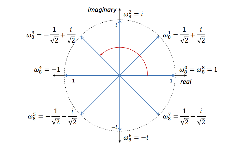
Consider a polynomial that requires 8 points as its value representation. In the first recursion, each input is squared, and according to De Moivre’s formula, this operation is equal to \(\omega_8^k=e^{ik\pi/4}\) rotating itself by \(k\pi/4\). Therefore, \(\omega_8^1\) lands on \(\omega_8^2\), \(\omega_8^2\) on \(\omega_8^4\), and so on. Eventually, after 3 recursions, every point would be superposed onto \(\omega_8^0\).
Evaluation (FFT)
The FFT algorithm could be outlined as:
For coefficient representation of polynomial \(P(x): [p_0,p_1,...,p_{n-1}]\), we define
\[\omega=e^{\frac{2\pi i}{n}}:[\omega^0, \omega^1, ..., \omega^{n-1}]\]The base case is \(n=1\rightarrow P(1)\).
Recursively evaluate the two polynomials:
-
\(P_e(x^2): [p_0,p_2,...,p_{n-2}]\), with inputs \([\omega^0, \omega^2, ..., \omega^{n-2}]\)
solving it gives outputs \(y_e=[P_e(\omega^0),P_e(\omega^2),...,P_e(\omega^{n-2})]\)
-
\(P_o(x^2): [p_1,p_3,...,p_{n-1}]\), with inputs \([\omega^0, \omega^2, ..., \omega^{n-2}]\)
solving it gives outputs \(y_o=[P_o(\omega^0),P_o(\omega^2),...,P_o(\omega^{n-2})]\)
Then, we know that
\[P(x_j)=P_e(x_j^2)+x_jP_o(x_j^2)\\ P(-x_j)=P_e(x_j^2)-x_jP_o(x_j^2)\\ j\in\{0,1,(n/2-1)\}\]Modify it with \(x_j=\omega^j, (\omega^j)^2=\omega^{2j}\):
\[\begin{align} P(\omega^j)&=P_e(\omega^{2j})+\omega^jP_o(\omega^{2j})\\ P(\omega^{j+2/n})=P(-\omega^j)&=P_e(\omega^{2j})-\omega^jP_o(\omega^{2j})\\ j&\in\{0,1,(n/2-1)\} \end{align}\]Because \(y_e[j]=P_e(\omega^{2j}),y_o[j]=P_o(\omega^{2j})\),
\[\begin{align} P(\omega^j)&=y_e[j]+\omega^jy_o[j]\\ P(\omega^{j+2/n})&=y_e[j]-\omega^jy_o[j]\\ j&\in\{0,1,(n/2-1)\} \end{align}\]Eventually,
\[y=[P(\omega^0),P(\omega^1),...,P(\omega^{n-1})]\]The pseudocode of FFT could be laid out as follows:
def FFT(P):
    # P = [p(0), p(1), ..., p(n-1)] coefficient representation
    n = len(p)                                 # assume n is a power of 2
    if n == 1:
        return P                               # P = [P(0)]
    w = [e ^ (2*pi*i/n) for i in range(n)]     # define omegas
    P_e, p_o = [p(0), p(2), ..., p(n-2)], [p(1), p(3), ..., p(n-1)]
    y_e, y_o = FFT(P_e), FFT(P_o)              # recurse into sub-problems
    y = [0, 0, ..., 0]
    for j in range(n/2):
        y[j]       = y_e[j] + w[j] * y_o[j]
        y[j + n/2] = y_e[j] - w[j] * y_o[j]
    return y
Interpolation (Inverse FFT, IFFT)
Return to the original problem of polynomial multiplication \(C=A\cdot B\): we can now evaluate \(A, B\) with \(O(n\log n)\) complexity, and then use the value representations of \(A, B\) to compute the value representation of \(C\) in no time. Now is the time to interpolate the representation back to coefficient representation.
Recall the matrix \(\textbf{P}=M \cdot \textbf{p}\):
\[\begin{bmatrix} P(x_0)\\ P(x_1)\\ ...\\ P(x_d)\\ \end{bmatrix} = \begin{bmatrix} 1 & x_0 & x_0^2 & ... & x_0^d\\ 1 & x_1 & x_1^2 & ... & x_1^d\\ ...\\ 1 & x_d & x_d^2 & ... & x_d^d\\ \end{bmatrix} \begin{bmatrix} p_0\\ p_1\\ ...\\ p_d\\ \end{bmatrix}\]Or,
\[\begin{bmatrix} P(\omega^0)\\ P(\omega^1)\\ ...\\ P(\omega^{n-1})\\ \end{bmatrix} = \begin{bmatrix} 1 & 1 & 1 & ... & 1\\ 1 & \omega^1 & \omega^2 & ... & \omega^{n-1}\\ 1 & \omega^2 & \omega^4 & ... & \omega^{2(n-1)}\\ ...\\ 1 & \omega^{n-1} & \omega^{2(n-1)} & ... & \omega^{(n-1)(n-1)}\\ \end{bmatrix} \begin{bmatrix} p_0\\ p_1\\ ...\\ p_{n-1}\\ \end{bmatrix}\]Or,
\[P(\omega^k)=\sum_{n=0}^{N-1}p_n e^{-\frac{2\pi ink}{N}}\]\(M\) is called Discrete Fourier Transform (DFT) matrix. Solving \({\bf p}\) for \({\bf p}=M^{-1}{\bf P}\) gives the coefficient representation.
Sometimes, the FFT in its core is the algorithm for calculating DFT matrices efficiently.
Solve \(M^{-1}\):
\[\begin{bmatrix} 1 & 1 & 1 & ... & 1\\ 1 & \omega^1 & \omega^2 & ... & \omega^{n-1}\\ 1 & \omega^2 & \omega^4 & ... & \omega^{2(n-1)}\\ ...\\ 1 & \omega^{n-1} & \omega^{2(n-1)} & ... & \omega^{(n-1)(n-1)}\\ \end{bmatrix}^{-1} =\frac{1}{n} \begin{bmatrix} 1 & 1 & 1 & ... & 1\\ 1 & \omega^{-1} & \omega^{-2} & ... & \omega^{-(n-1)}\\ 1 & \omega^{-2} & \omega^{-4} & ... & \omega^{-2(n-1)}\\ ...\\ 1 & \omega^{-(n-1)} & \omega^{-2(n-1)} & ... & \omega^{-(n-1)(n-1)}\\ \end{bmatrix}\](somehow, apparently)
So
\[\begin{bmatrix} p_0\\p_1\\...\\p_{n-1}\\ \end{bmatrix}= \frac{1}{n} \begin{bmatrix} 1 & 1 & 1 & ... & 1\\ 1 & \omega^{-1} & \omega^{-2} & ... & \omega^{-(n-1)}\\ 1 & \omega^{-2} & \omega^{-4} & ... & \omega^{-2(n-1)}\\ ...\\ 1 & \omega^{-(n-1)} & \omega^{-2(n-1)} & ... & \omega^{-(n-1)(n-1)}\\ \end{bmatrix} \begin{bmatrix} P(\omega^0)\\P(\omega^1)\\...\\P(\omega^{n-1})\\ \end{bmatrix}\]This is very similar to \(\textbf{P}=M \cdot \textbf{p}\), except we replace \(\omega=e^{\frac{2\pi i}{n}}\) with \(\omega=e^{-\frac{2\pi i}{n}}\), and then divide the whole matrix by \(n\). So, the pseudocode for IFFT is can be straightly copied from FFT, with some minor edits:
def IFFT(P):
    # FFT ---> IFFT. Except here the input P is the value representation and
    # output y is the coeff representation.
    n = len(p)
    if n == 1:
        return P
    w = [e ^ (-2*pi*i/n) for i in range(n)]     # w = w ^ {-1}
    P_e, p_o = [p(0), p(2), ..., p(n-2)], [p(1), p(3), ..., p(n-1)]
    y_e, y_o = IFFT(P_e), IFFT(P_o)             # recurse into IFFT sub-problems
    y = [0, 0, ..., 0]
    for j in range(n/2):
        y[j]       = y_e[j] + w[j] * y_o[j]
        y[j + n/2] = y_e[j] - w[j] * y_o[j]
    return y

# then, outside of the recursion, divide the result by n = len(p).
And this is the full picture of Fast Fourier Transform.